Introduction

Recommender Systems

The main goal of a recommender system is to provide users with hints and suggestions about items that can meet their interest.

The Internet, today, provides a large variety of examples: hotels recommended by Booking-dot-com, books recommended by Amazon, songs by Spotify, movies by Netflix, and many more.

1. Recommender systems algorithms need, as their main input, a set of available items (e.g., books, movies, hotels), enriched via a set of descriptive attributes. For the example of movies, these attributes could be: title, year of release, genre, director, actors, etc.
2. Recommender systems algorithms, beside the “items”, need to know about “users”, since each recommendation aims at an individual user. Demographic data, like age, nationality, gender, area of living, are possible attributes to describe a user. In addition, algorithms need to know about user preferences. For example (for movies): science fiction (genre), Harrison Ford (actor).
3. A third type of information that characterizes a user is the how she interacts with items: for instance, a user may have rated some movies. In this case, we explicitly know the opinion of the user of these movies. Alternatively, we may know which books a user has bought in the past, or which movies a user have watched. We can implicitly assume that, if a user watched a movie or bought a book, probably the user likes that movie or that book. Similarly, if a user stopped watching a movie after 5 minutes, we can implicitly assume that the user did not like that movie. Interactions have attributes as well. These attributes are called “the context”. Example of contextual attributes are: people, time, and weather.

The same user may have different opinions on the same item, based on the context. For instance, when choosing a restaurant for dinner, the choice could be different if the user is planning a business dinner or a romantic dinner. Similarly, if the weather is sunny, the user might prefer a restaurant with an outdoor garden, while if the weather is cold, the user might prefer a restaurant with a fireplace.

Data Representation: ICM&URM

Data representation. We examine now how to represent the input for recommender systems. The ICM, Item Content Matrix, represents a table where each row is associated to one item, while each column corresponds to one attribute. In the simplest form, the possible values in the matrix are 1 (if the attribute-value belongs to the item) or 0 (if the attribute-value does not belong to the item). If, for example, actor “x” plays in the movie “y”, the value would be 1 for the row-corresponding to “y”, at the column corresponding to “x”.

In a more sophisticated version, the value are real numbers expressing the relevance of the attribute-value for the item. If an actor, for example, plays the major role in a movie, he may get value 1.0. If he plays a medium role, the value could be 0.5. Another important matrix is the User Rating Matrix: in the user rating matrix, rows represent users, and columns represent items. Numbers represent ratings assigned by each user to each item, either implicitly or explicitly.

Taxonomy of Recommender Systems

This section takes into account three points: categorizing algorithms, content-based filtering and collaborative filtering.

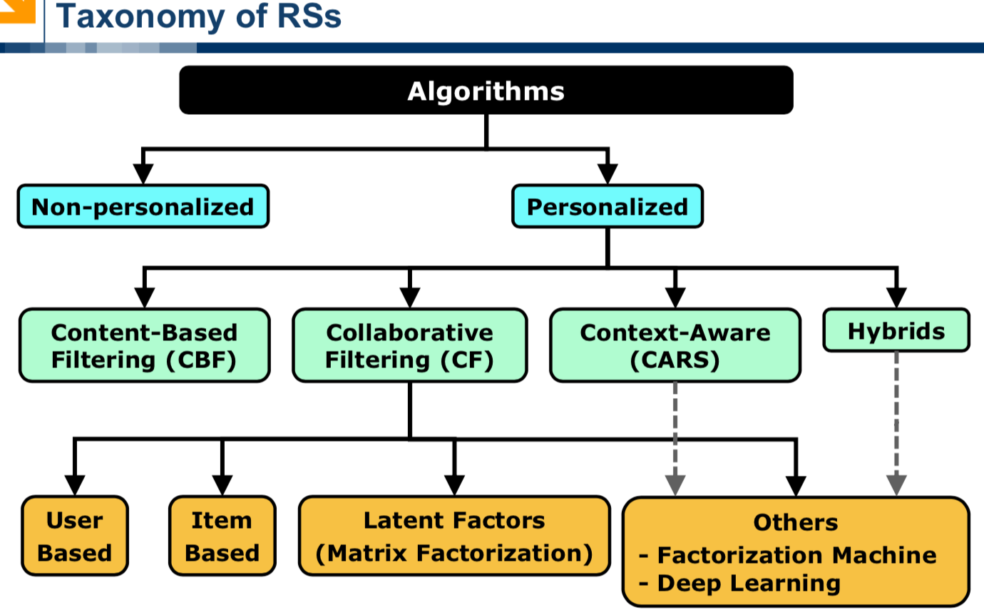
Categorizing algorithms

Recommender algorithms can be classified into two categories: personalized and non-personalized recommendations. With non-personalized recommendations, all users receive the same recommendations.

Examples are: the most popular movies, the recent music hits, the best rated hotels. With personalized recommendations, different users receive different recommendations.

The focus of this course is on personalized recommendations, although we will use non-personalized recommendations as baselines. The core idea for personalized recommenders is that they make “better” recommendations than non-personalized systems. However, we will see that there are some scenarios in which non-personalized recommendations are still a good choice.

For instance, if you recommend the most popular movies, by definition, you will recommend movies that most users like.

Techniques for personalized recommendations can be further classified in a number of different categories. The most important are: Content-Based Filtering and Collaborative Filtering.

Content Based Filtering

The basic idea with Content-Based recommendations is to recommend items similar to the items a user liked in the past.

For instance, if you liked the movie “Indiana Jones”, the recommender system could recommend you other movies directed by the same director (Steven Spielberg), and/or with the same main actor (Harrison Ford). As a second example, when you are looking at a page describing a product on the Amazon web site, you receive recommendations listing products similar to the one you are looking at.

Content-Based filtering has been one of the first approaches used to build recommender systems. One important prerequisite for Content-Based filtering to work is to have, for each product, a list of “good quality” attributes (such as genre, director, actors, in the case of movies). We will see later in the course what makes an attribute a good attribute.

Collaborative Filtering

Collaborative Filtering techniques do not require any item attribute to work, but relay on the opinions of a community of users. The first type of collaborative recommender system invented was based on user-user techniques (or user-based techniques). The basic idea is to search for users with a similar taste, that is, users sharing the same opinion on several items.

As an example: if Bob and Alice have the same opinions on many movies, it is likely that, if Bob likes a movie, also Alice will like the same movie.

This idea seems reasonable, but we will see later in the course that the user-user approach doesn’t always work well. In many scenarios, user-based techniques fail to provide good recommendations, or are not able to provide any type of recommendation at all.

The second type of collaborative recommenders are item-item or item-based algorithms.

Item-item collaborative filtering was first invented and used by Amazon.com in 1998. The basic idea is to calculate the similarity between each pair of items according to how many users have the same opinions on the two items.

For instance, if most users who liked “Indiana Jones” also liked “Star Wars”, it is highly probable that a user who likes “Indiana Jones” will also appreciate “Star Wars”. Many commercial recommenders today rely on item-item algorithms.

During the Netflix competition, a new family of collaborative filtering algorithms has been invented, based on a technique called matrix factorization, which is part of a more general family of algorithms called dimensionality reduction. Contrary to user-user and item-item algorithms, it is not easy to provide an intuitive explanation on how algorithms based on matrix factorization work.

Ratings, Predictions and Recommendations

“Explicit rating” means that the user explicitly states her satisfaction with an item (typically using a 1 to 5 scale). Ratings by users are a very important input for recommender systems.

In many application scenarios, however, it is not possible (or advisable) to ask for the opinion of the user. Rating by users may be difficult for different reasons. Users are not always happy to “waste” their time with ratings. Annoyed users may provide “random feedback”. And, in fact, frequent rating requests may annoy users. (Reminder: when designing a Recommender System, it is important not to annoy the user with too many requests!). Some technologies do not allow to easily collect explicit ratings by the users (for example, traditional TV).

“Implicit rating” is an important alternative to explicit rating. Implicit rating attempts to “guess” the opinion of the user. For example: you buy a book from Amazon. I don’t know if you liked it. But I know that somehow you did something with it. I can assume that if you buy a book, probably it’s because you like something in the description, you like the story. I can assume that if you buy a product you like something in that product.

This assumption is not always true. Sometimes, the user buys a product, tries it, and is not happy about it. If there are no other options available, however, we’re obliged to make this assumption. Another example. Assume that Mary (a user) buys a movie on Netflix. We may assume, in general, that she likes that movie (since she bought it). If, however, Mary stops watching the movie after a few minutes, we may assume that she did not like it.

But this assumption could be true in general (and therefore statistically valid in the end), but wrong in specific cases (the user may have received a phone call, for example). For various reasons, implicit ratings are more reliable when applied to positive ratings (what users like), rather than to negative ratings (what users don’t like).

Inferring preferences

This section describes the characteristics of the formal representation of input and discusses about the sparsity of User Rating Matrix.

Formal representation of input.

Implicit or explicit ratings can be collected in various way. In the following, we will discuss how to use ratings, independently from the way they were collected.

Let us assume that implicit ratings are in a scale from zero to one. Zero means you have no information. (be careful, not a bad rating but no information!). 1 means that a user is perfectly happy with the item.

More formally, URM (User Rating Matrix) is a matrix where each row represents a user and each column represents an item. rui is value for the row corresponding to user, “u”, and the column corresponding to item, “i”.

URM (or something similar) is the main input of almost all recommender systems. URM, however, is almost never implemented as a matrix, this matrix could be huge (and with too many 0 in it). Very very SPARSE.

Nonpersonalized Recommenders

“Non-personalized” recommender systems suggest the same items to all users. The easiest and best way to make non-personalized recommendations is to recommend the most popular items.

1. “Most Popular” items are those who have most ratings (whatever is their value);
2. “Best rated items” instead are those with the highest average values of ratings.

In order to compute “popularity”, recommender systems have to count the number of zero elements of the columns. After counting all the non-zero elements for each column, we can take the columns with the highest result and those will be “the most popular items”.

There is a contradictory situation with popularity: the positive side is that users are likely to like the items recommended; the negative side is that there is little added value, since it is likely that users were already aware of those items.

“Best rated” items have the highest average ratings; they are, for non-personalized recommendations, an alternative to most popular items.

To compute the average ratings, we may use the standard notion of average; but in reality this does NOT work very well. The problem is that an average computed over several ratings is much more reliable than an average computed over a few ratings.

For example: suppose that there is one restaurant which has only one rating. If the rating is 5, it may have been solicited by the owner. If the rating is 1, it may have been solicited by a competitor. In both cases the “average” is not a reliable measure.

The number of users who rated an item is called the support; ratings with high support are more reliable than ratings with low support.

Scales and Normalization

In this section, we discuss about scales and normalization, taking into account ratings distribution and computing ratings.

Ratings distribution.

In a typical scenario, in a scale 1 to 5, most of the ratings have value 3, and besides that, most of the ratings will be positive and there will be very few negative ones.

Normally, people are more easily convinced to rate something if they liked it. Users are more willing to share their experience for products they liked and less for products they didn’t like. If we plot the distribution of ratings about all items (including good and bad ones) most users give a rating between 3 and 5. Very few users give ratings 1 and 2.

This distribution doesn’t reflect the distribution of the quality of a product, and probably does not even represent the opinion of the users. It is somehow related to the way people are used to rate products: most users do not bother to provide negative ratings, while happy users are willing to share their experience.

Computing the ratings.

Let’s suppose we want to compute the average rating of the item “i”,”bi” is the average rating of product “i”.

The simple definition of the rating an item “i” is: “The Average Rating of an item is equal to the sum of the received ratings divided by the number of received ratings“

NU is the number of rows (for the column corresponding to i) with value other than 0, i.e. the number of users that have provided a rating. If very few users (or only one) has given a rating, this is not a reliable measure.

We can improve the reliability with the trick of adding a constant, shrink term, C at the divider.

“The Average Rating of item is equal to the sum of the received ratings divided by the number of received ratings plus a shrink factor”

If NU is high, the average will not be much affected; if NU is small, the average will lower significantly.

For Example: Suppose we have two restaurants; one of them has 1 rating equal to 5; another one has 100 ratings, all of them 5. Without using a shrink term, both restaurants have the standard average rating of 5. Using a C=10 instead, the first restaurant has an average of 0.45 and the second of 4.54.

The shrinking term is a crude technique that helps to take into account the bias implicit when there are only few ratings for one item. There are more sophisticated approaches, but often they generate results quite similar to those obtained with the shrinking term. A

nother Example: Check on some recommender systems (e.g. Trip Advisor): you may verify that, for items with few ratings, the overall rating of an item is not based on the standard mathematical average.

Global Effects

This section describes the so-called algorithm global effects, giving a general overview and showing how to compute averages and biases.

General description.

The “global effects” technique is very important for two reasons:

1. It is a non-personalized formula which is able to provide good quality recommendations.
2. Secondly, it is a building block for much more sophisticated techniques. And, in fact, advanced personalized techniques do not work well, unless we combine them with global effects.

Here is the key idea: normally, most of the users tend to give (almost) the same ratings to different items.

Let’s show how in an extensive example: in order to detect “good movies” we can compare the average rating of each movie with respect to the average rating of all the movies. Now suppose that the average rating for all movies is 3.5. If a movie has an average rating of 3, it means that the quality of this movie is less than the average, while if it is 3.8, the movie is better than average.

Computing averages and biases

There are six steps to be considered.

1. We compute the average rating of all the movies. For each item, we sum together the rating given by all users for that item; then, we add these sums for all items; then, we divide by the number of explicit ratings other than zero. Zero means we have no information (it is not a bad rating).
2. We compute now for each non-zero rating a new normalized rating, subtracting the average computed in step one to the rating itself. So, if an item was rated four by the user, and the average rating for all the items is three point five, the new rating is 0.5. Applying this rule to all ratings (other than zero), we compute a new URM removing the global effect.
3. Now we compute a different rating for item by adding up all the normalized ratings by all users and dividing by the number of users who gave a rating. This new value is called the item bias: it tells us the bias of that item with respect to all items.
4. We compute yet another rating, creating a third version of U R M. For each item, we subtract the item bias from each normalized rating, obtaining another rating.
5. For each user, we compute the user bias. This is the sum of all her ratings (using the version we have computed before) divided by the number of items for which the user has provided a rating. This step takes into account the fact that different people have psychologically different rating scales. Some people are very nice, optimistic people, so if they do not like something, they give a rating of four, while there are some other users that are not friendly and if they like much a product, they give three.

   Here is a funny example of a user bias: I was reading the reviews on Trip Advisor about a luxury hotel and there was a review from a user who gave a rating of two out of ten: the user was complaining because the coffee machine in the room was not an “Espresso” but it was of another kind. So, according to this user’s opinion, the score for the hotel would be two. This user probably was giving very low ratings to all the hotels. This is an example of a user bias.

6. Step six: the final rating of user for item can be computed adding the three elements: overall average (for all items and all users) plus the item bias plus the user bias. This is the final formula for the Global Effects.

Recap:

1. Compute the average of the ratings (μ) from URM.
2. Remove this quantity from the URM.
3. Compute the average for each item (b_i).
4. Remove this quantity from the URM.
5. Compute the average for each user (b_u).
6. Compute new rating, summing the average of ratings to the item bias to the user bias.

So now we have 3 terms: “u” is a scalar, “b_i“ is a vector (1 for each product), “b_u“ is a vector (1 for each user). This way, we can estimate the rating a user would give to an item.

This is not exactly non-personalized, because there is a term that depends on the user. Each user is receiving a different estimation. Technically speaking, this should be considered as a personalized recommendation, but since this technique is computed in a very basic way, by just computing the average, it is often classified as a non-personalized recommendation.

Requirements

This section presents basic concepts about requirements for recommender systems.

Functional vs. non-functional requirements.

For all pieces of SW there is an important distinction between functional requirements (what the SW does) and non-functional requirements (how the SW does its job).

It is clear that functional requirements have the priority, since if a piece of SW fails in performing its functions, it is useless. It may happen however, that the piece of SW, although it fully satisfies functional requirements, it is not acceptable, because non-functional requirements are not adequately satisfied.

Non-functional Requirements

1. Response time: Response time is a crucial non-functional requirement, since even the best recommender system would not be acceptable if the it takes too much time to get the recommendation. A concrete example: recommendations shown in webpages of online shops must be very fast; it is accepted today that users do not wait for a page to load more than 4 sec. If the recommender systems slow down the loading of the page, it will become useless or even negative.
2. Scalability: Scalability is an important non-functional requirement for recommender systems. Environment like Netflix, Amazon, or Google need to manage millions of users and to catalog millions of items. Millions of products. Recommender systems need to be scalable in the sense that coping with growing users can be accomplished by simply adding new computers in the data center. If applications are not scalable, however, adding new computing power will not help.
3. Privacy and Security: Privacy and security are important non-functional requirements. Regulations dictate that data about users and their behaviour need to be protected, and not accessible to outsiders. General regulations exist everywhere; in Europe we have European guidelines and national regulations. A typical concern is about reverse engineering; recommendations are often based on past actions of users; it must be prevented that outsiders can steel information about recommendations and from there can induce the behaviour of users.
4. User Interface: The interface of a recommender system, is a very important nonfunctional requirement. One example. What is the best moment to show a recommendation? As soon as the user logs in into the system, or when she is surfing in the catalog of products, or when she is reading the description of a product, or when she is doing the checkout? Also, how many products, how many items should be shown to the user? One, two, five, 10? Also, how should recommendations be shown to the users using stars? (one to three, one to five, one to 10?). Thumbs up thumbs down?

Quality Overall

A recommender system needs data in order to provide recommendations. Data about users, data about items, data about attributes describing the items, etc.

If data are faulty, or missing or incorrect, the quality of a recommender system will be poor. The quality of algorithms for providing recommendations is a main concern of this course; we should be, however, of the relevance of the other aspects.

Experimental data indicate that the quality of algorithms count for 20% (more or less), of the total quality perceived by the user. So designing a full environment of a recommender systems (from data to the user interface), the designer should balance the effort across the various elements, being aware that algorithms are just a part of the whole system.

Quality Indicators

1. Relevance and Coverage: Relevance is the ability of recommending items that very likely most users will like. One way to design a good recommender in terms of relevance is to never recommend those products that few people like. Coverage is the ability of recommending most of the items of (a possibly very large) set of items. Coverage is the percentage of items that a recommender system is able to recommend. Recommender systems with high relevance, may have a low coverage (since they recommend items that most users like), and vice versa.
2. Novelty and diversity: Novelty is the ability of recommending items unknown to the user. Recommending new items (e.g. new restaurants or new books) may be an added value for he users. Diversity is the ability to diversify the items recommended. If the user has known preferences (say that she likes chines restaurants or science fiction movies) it is safe to recommend items corresponding to the taste. But it can be boring, so it could be wise sometimes to “diversify” recommendations.
3. Consistency and Confidence: Consistency is about the stability of the recommendations. Some recommender systems are very dynamic, continuously updating the user profiles, and therefore modifying their recommendation. An example: the recommender system suggests movies “x” and “y”. Assume that the user watches “x” and rates it very high. The recommender system may update her profile and exclude “y” from next recommendation. This inconsistency may confuse the user. There are some recommender systems that can be too dynamic in their behavior. Confidence is the ability of measuring how much the system is sure about a recommendation. A confidence of 100% is practically impossible. What is the proper level of confidence? 90%? 60%? Is it wise to recommend an item with a level of confidence not very high? (may be for increasing diversification)
4. Serendipity: Serendipity is the ability of “surprising” the user surprise you. Surprising means to recommend something unusual for the user, who can “discover” something unexpected. A recommender algorithm is serendipitous if it recommends something that the user would never be able to find or would never search for.

Evaluation Techiniques

1. Direct User Feedback: ask some real users to define their level of satisfaction.
2. A/B Testing: Compare the behaviour of the users who receive recommendations with the behaviours of the uses who do not receive recommendations(如：收到推荐的人是否购买的product增加了？)
3. Controlled Experientments: Use NOT real-life users to test the satisfaction and give feedback.
4. Crowdsourcing: asking volunteers to answer online questionnaire.

Offline Evaluation

Above the evaluation techniques we talked about are online evaluations, which evolve real users or models like real users. now we talk about offline evaluation.

1. Ground Truth: Let us assume that several users (say 100000) have expressed their opinion about several items (say 10,000). In reality each user expresses an opinion about a few items, and each item is reviewed by few users. We call “ground truth” the opinion of the users about the items. In the field of recommender system there is the adoption of a peculiar terminology: we call “relevant opinions” the positive ones, and “relevant users”, those who have expressed them. The other users are the irrelevant ones.
2. Top-K recommendations: Let us assume that a recommender system computes in a given situation, for a given user, which products to recommend. We call “top-K” recommendation, the K items that the recommender system predicts to be liked most by the user. In order to assess the quality of the recommender system, we need to compare top-k recommendation with the ground truth, that is, opinions expressed by the users.
3. Error metrics: We use the “error metrics” to measure the difference between the rating estimated by a recommender system and the true rating provided by the ground truth. Given a user and an item we can ask the recommender system to provide a rating: say 7 out of 10, for example. Let us assume than the rating in the ground truth (for that user and that item) is 4. The difference between the two ratings is 3.
4. Classification metrics: Classification metrics assign a label to items. Let us assume that the recommender system has recommended 10 items. Some of them (let’s say 3) are actually liked by the user. Some of them (let’s say 2) are disliked. For the other items (let’s say 5) we have no opinion by the user. Generally speaking, we have four sets to consider: A, B, C, D. A is the whole dataset. B is the set of items that the user likes. C is the set of items that the user doesn’t like. D is the set of items that we are recommending.
5. Advantages and disadvantages: The fact that for some items there is no opinion of the users, is a disadvantage for error metrics. If some of the items belonging to D(recommended items), do not belong to either B(liked items) or C(disliked items), we can’t compute a difference in ratings. Error metrics, in fact, despite being very popular, not always provides a good indicator of the quality of a recommender system. In the field of recommender systems, both methods can be uses: error metrics or classification metrics. Still, the fact that some items are not rated by the users create methodological problems.

Algorithms

Recommender Algorithm

A recommender algorithm is a mathematical function. The input is the URM. The output is what we call the “model”, that is, a representation of the user preferences.

Recommender algorithms above described, are based upon two functions, F (build a model) and G (use the model); they are called model-based algorithms. With memory-based algorithms, instead, there is no model. The algorithm uses past data to provide recommendations. A memory-based recommender system is able to provide recommendations only to users that exist when you build the model. It is not able to provide recommendations to other users. Normally, memory-based algorithms provide better recommendations. But they are slow and therefore do not scale easily.

Relevant Data Sets

1. The first dataset is the one used to build the model, that is, a guess of the taste for each one of several users.
2. The second set is about other users; the model is used to forecast the taste of these users.
3. The third dataset is created comparing the estimated ratings with the actual ratings provided by the users

Evaluation Techniques

Hold-out techniques

Let us consider the URM. The hold-out technique randomly removes some of the ratings from the matrix. The best practice is to remove, more or less, 20% of the ratings. The model is computed (function F) and recommendations are generated (function G).

Then the estimated ratings are compared with the true ratings that were removed. Though it is very popular, this technique is not an optimal one; one of the disadvantages is that you can evaluate the recommendations only for the users that are both in the training set and in the hold-out set.

K-fold evaluation

This technique partitions the URM in 3 portions, by selecting different users (and therefore different rows). One portion (obtained by selecting some users) is used to train the model. Two other portions are used to verify the quality of the recommendations.

It is important to notice that, while hold-out technique randomly removes ratings, k-fold evaluation removes all the ratings of some users. This technique is more difficult to implement: it is also difficult to test the quality of recommendations

Leave-one-out technique.

When you use hold-out or K-fold, our sparse dataset represents a big problem because, for each user, we have just few ratings, but the average is still very low.

Suppose, using hold-out, you take the user Paolo Cremonesi who rated only four products on Amazon. If we randomly remove only one rating from the user, we have three ratings that we can use to build his model and to understand his taste. So, we evaluate the quality of recommendations to a user, by using only one product and the only way to compare the quality of the recommendation is by comparing the true opinion of Paolo with the estimated opinion. Unfortunately, we can’t trust too much this rating. Now, suppose you remove three ratings from Paolo Cremonesi, using them to analyze the quality of the recommendation. However, there is only one rating that we can use to understand the user’s taste, not an easy way to realize the opinion of a person. So, because the number of ratings per user is normally very low, when you split your dataset you have not enough rating to keep the profile alone and to do a statistical significant quality measurement.

By using leave-one-out, from one user profile you create four profiles by removing one rating, using it for testing. This technique, always used in normal situations, is not only a nice trick to try to solve the problem of having few ratings in the user profile, but probably also the best way to remove ratings.

Despite that, few people do it for a number of reasons. Firstly, it is difficult and boring to implement. Furthermore, it takes much more time to do the testing because you need to remove and reset, continuously. Clearly, if you have a dataset in which your users have a lot of ratings or your users on average have hundreds of ratings, you do not need leave-one-out.

Error Metrics

1. Mean Absolute Error: For each rating, the absolute value of the difference between the actual rating and the estimated rating. The overall average is the MAE.
2. Root Mean Square Error: The Mean Square Error consists in computing the average of the squared difference between each actual rating and the estimated rating. Often, for normalization, the square root of the result is considered. Minimizing the root mean square error is (relatively) easier than MAE.

Limitations of error metrics.

There is an intrinsic problem: algorithms compute ratings for all items, but users only rate a few items, therefore it is not possible to compare the computed rating with the actual rating by users. In addition, users normally tend to rate items that they like. Typical distributions of ratings show this phenomenon; there are very few ratings for items that the users do not like.

Comparing the distributions of ratings

Users, in general, take at items only if they have, at least, a mild interest for them. If we could have all users rating all items, the percentage of negative ratings would be much higher.

Assumption of error metrics

In essence the error metrics assumes that ratings are missing at random. This is why the quality measure with error metrics is not a good indicator of the quality of a system. Because in reality the missing ratings would much more negative than the available ratings.

Classification metrics

Recall

The recall is the ratio between the number of items recommended (say N) and the number of items that the user would actually like (say K). If recall (N/K) is low, it means there a lot of possibly good items that we are not recommending. If the ratio is high, it means that the system is recommending most of the possibly good items.

Precision

Precision. Let us assume that the system recommends N items, and that X of these items are actually good for the user. “Precision” is the ratio between X and N. High precision means that most of the recommended items are good for the user; low precision means that several recommended items should have not been recommended.

Recall and Precision are in general at odds, in the sense that optimizing recall may lead to a low precision, and viceversa. If the system, for example, recommends only the best item, precision is 100% but recall is very low. If the system recommends a lot of items, recall will be very high, but many of the items could be wrong, therefore the precision could be low.

Balancing Precision and Recall may be difficult, since both of them are important. For recommender system, overall, recall is (slightly) preferred; it is better to not miss any good items, even if the price is that some bad items come along.

Fallout

Fallout is another important metrics. It is defined as the ratio between the bad items recommended and the total of items with poor rating by that user.

Combining metrics

Precision or recall?

Recall is the most important metrics for Recommender systems. Despite this, recall, by itself is not sufficient, but it must be combined either with precision or with fallout. When we examine together precision and recall, we must take into account the value of N, that is, the number of items being recommended.

A perfect recommender system has precision of 100% for all the values of recall. In reality however, for a large N we increase recall, since more good items are recommended, but precision decreases, since some of the items are not really relevant for the user. For a small value of N, most of the items recommended are relevant for the user, but some of the possibly relevant items are not recommended.

F-Measure: combining precision and recall.

F-measure is defined by multiplying “precision”, “recall” and the constant value 2.

ROC Curve

Plotting together Recall and Fallout, we obtain what is called which is called the ROC curve. Increasing the Value of N, recall increases, but also Fallout increases. If all the items are recommended, both recall and fallout have the maximum possible value. In practice however, recommender systems are interested only in small values of N.

In addition, measuring Fallout is not always possible; In an “implicit dataset” only the ratings by the user are represented, and the negative ratings are in general missing.

Fallout can be computed only if the negative ratings are explicitly defined. In order to summarize the ROC curve in a number, the area under the green line is computed. This number is called AUC(the area under the curve). For a perfect recommender system, the value of AUC will be one.

Popularity bias.

It is easier to collect opinions for items that are very popular and more difficult to collect opinions about items that the people do not care of. This create a problem called “popularity bias”.

Utility.

Utility measure the value provided by a recommender algorithm. Recommending the most popular items, it is very likely that the user likes the recommendation; but it is not very useful, since the user is (probably) already aware of those items.

A useful recommendation combines two facts: the user likes the recommendation and the user gets something new. One possibility is to remove from the test set the most popular items.

In an experiment we removed some of the most popular movies in Netflix: something like 60 movies out of 12,000 movies. As shown by the picture, the quality of the top popular items is the worst. So, generally when you are evaluating a recommender system you should build the test set by taking into account the popularity bias.

Ranking Metrics

Ranking in general.

Classification metrics have the goal to determine if a user likes an item or not. Ranking evaluation metrics, instead, try to measure how much a user likes an item, compared to the other items.

In practice, ranking metrics are used when an order list of recommendations is presented to the users. Generally speaking, when presenting to a user a list of items, it is advisable to put high in the list the items that the user likes most.

So, in principle, a ranking algorithm, given two items, X and Y, should rank them, putting higher in the list the most liked one. In other words, the list of recommendations will present the most relevant items at the top, and the least relevant items at the bottom.

Average Reciprocal Hit-Rank.

The Average Reciprocal Hit-Rank, ARHR, is a modified version of recall. Recall, is defined as the number of items that the user likes, included in the recommendation, divided by the total number of items that the user likes.

With this technique the denominator is the same. For the numerator each item is “weighted” by a fraction: 1 divided by ranking, that is, the position in the list. The weight is equal to 1 if the item is in position 1; 0.5 if the item is in position 2; and so on.

This is a useful metrics, but technically speaking is not a ranking in strict sense, since it does not compare the ranking provided by the user with the ranking provided by the system.

Mean Average Precision.

The Mean Average Precision, or MAP, is a very important metric. With MAP we compute the average precision across several different levels of recall.

Precision and recall are computed for each item added to the list of recommended items.

In practice the first move is to take the first item: precision is 1 since the user likes the item; recall is 1/100, assuming that there are 100 items that the user likes. Let us consider the second item. Precision is again 1, if the user likes also the second movie. Recall this time is 2/100.

When K = 2 we can compute DELTA-R, is equal to the difference between the last recall, 2/100 and the previous one, 1/100. In order to compute the MAP for a value of K, we multiply the precision for each value of P(i) for DELTA-R.

Spearman’s Rho.

Spearman’s Rho coefficient measures the consistency between the ranking as provided by the system and the ranking as provided by the user. It is considered a global ranking metrics, in the sense that all items are considered. Ranking items in a list means that the user puts them in a specific order: the first is the one the she likes most. The Spearman coefficient is 1 if the ranking of the system of exactly corresponds to the ranking provided by the user.

Kendall’s Tau.

The Kendall’s Tau metric considers pairs of items, not individual ones. Let assume that we have two list of 10 items. There are 45 possible pairs; for each pair the user ranks it (which of the 2 does she prefer?) and the system ranks it. The pair is Consistent if User and System have the same opinion; it is Discordant otherwise.

In addition, we must consider the number of pairs for which the user could not express a preference; and analogously for the system. The Kendall Tau metrics takes into consideration these 4 numbers: consistent pairs; discordant pairs; pairs not ranked by the user; pairs not ranked by the system.

Kendall’s Tau limitations: Kendall’s Tau closely represents the opinion of users, and therefore is a good technique. A major problem is the time required for computing it.

Evaluating Diversity

Defining diversity.

There are several possible definitions for the notion of “diversity”.

1. “Intra-list diversity” means that all the items within the same list are quite different.
2. “Extra-list diversity”, means, instead, that the items in two different lists are different. This can be useful for two consecutive recommendations.

Measuring distance

How is it possible to measure the dissimilarity between two items? Let us consider the attributes used to describe an item: for a movie they can be the actors, the genre, the director, etc. For a pair of items, if they have several attributes in common, they are similar; otherwise they are dissimilar. If no attributes are in common, they have the maximum distance.

Balancing quality and diversity.

A good recommendation system should balance quality (recommending items that users like) with diversity (recommending dissimilar items).

Playing “conservative” a recommender system may choose very similar items, improving precision, but probably lowering diversity. As it can be seen on the slide, improving diversity may decrease precision, and viceversa.

Evaluating Novelty

Defining novelty.

Novelty is another important metrics. The definition of novelty: number of recommended relevant-and-unknown items divided by the number of relevant items.

Estimating novelty.

Recommending a very popular item, there is the danger that the item is already known by the user. While recommending an item that is not popular, the probability that this recommendation is novel is very large.

A good approximation of novelty is the following. By popularity we mean the percentage of users who rated an item. The reciprocal popularity of an item is 1 over the popularity.

A way to improve the novelty, consists in using “diversity”. If the dissimilarity, between the movies recommended and the movies that the user watched in the past, is high, probably the novelty is also high.

Content Based Filtering

Definition

CBF is to estimate how relevant an item is for a user, based on the items for which they have previously expressed a preference.

Basic Logic: If a user expressed a preference for an item, it is likely that he will like similar items.

ICM - Item Content Matrix

ICM is the fundamental of CBF. Each row represents an item and each column an attribute. And the value ranging from 0 to 1 in most cases.

Cosine Similarity

The simplest way to measure the similarity between two items is to count how many attributes they have in common.

If the item-vector are binary with 1 and 0, we could say that the product of two vectors could be a good measure of the distance between two items.

The cosine

Counting common attributes is not meaningfult if we are not working with binary values. Cosine similarity is the simplest way to measure the distance, by taking the dot product of item i and item j and dividing them by the product of the norm of the two items.

The result measure the angle between two vectors. If the result is close to 1, it means two vectors are quite close (similar).

Shrinking

PROBLEM: there are many cases in which we do not have the attributes or we have few of them. This represents a problem for computing the cosine similarity.

eg: 两部完全不相同的电影，同一个演员客串了非常小的一部分，且ICM只有一列，就是客串演员，显然两部电影的cosine similarity是1，但是这是与事实相悖的。

A useful trick is to add a constant value (shrink term) in the denominator of the cosine similarity formula.

By adding a shrink term, we increase the reliability of our similarity. That means, that if we have a similarity close to one, we are sure that there are several attributes in common between the items, therefore we can trust that the items are actually similar.

Estimating ratings

PROBLEM: 当user对于多个（可能有很大差别的）item有一定的preference时，如何进行recommendation。

GOAL: estimate how much user “u”, likes an item “i”, a item. The only information that you have is his opinion about other items “j”.

The simplest estimator, is the weighted average of the previous ratings, using the similarity between the item “i” and items “j” as the weight.

new_item_estimated_rating = SUM(previous_item_similarity*previous_item_rating)

EG: You know that Bob likes The Matrix and rated it 5 stars. He also likes ‘Forrest Gump’ and rated it 4 stars. We want to estimate the rating that Bob gives to ‘Star Wars’. We average these rating, giving more weight to ‘The Matrix’ since it shares a similar genre and themes with ‘Star Wars’, and giving very little or no weight to the rating of ‘Forrest Gump’, a very different kind of movie.

Similarity Matrix

To build CBF, it is useful to build similarity matrix. Each row are items, and each column are items. The value is the similarity between different items.

Similarity Matrix is sparse and really big. The solution of this is take k-nearest neighbors. It means instead of keeping all the matrix, for each item(row) we only keep k most similar items.

Choice of k:

If “k” is too small, we get a very low quality, because you don’t keep enough similarities to compute an appropriate estimation. As you increase k, you have a better quality.

Then, if you go on increasing “k” too far, the quality start decreasing, because you are polluting the estimation with items that are not relevant to estimate the opinion of the user.

Improving ICM

A standard good quality Content Based Recommender System estimates the rating a user would give to an item, based on cosine similarity improved with the shrink term, and considering the k-nearest neighbors.

1. Non-binary values: Sometimes it is more accurate to have values in between zero and one, especially when one attribute only partially describes an item.
2. Attribute weights: How do we weigh each attribute? Based on how much important is an attribute in the ICM, the results of recommendation will be different.(eg:what kind of sandwiches provided by the company to the actors during the break time is totally useless for a user to choosing a film!)

TF-IDF: Term Frequencies - Inverse Document Frequencies

Very often attribute is a piece of text written by anyone. It seems more a NLP problem, but we still have to solve this.

One possibility is that the keywords or tags generated by the users in the summary is an attribute. But to weight this attributes, we need to use TF-IDF. (Yes! The TF-IDF Technique used in NLP!)

attribute weight=TF/IDF

Term Frequency

KEY IDEA: if a word appears a lot of time in a document, probably this term is important to describe the document. Term frequency is how many times specific term appears in current text.

Inversed Document Frequency

IDF is computed as the logarithm, on any base you want, of the ratio between the number of items that are present in the data set divided by the number of items that contain attribute a.

If attribute “a” is present in all items, you have the number of items in the catalog divided by the number of items that contain attribute “a”: the ratio is 1 and its logarithm 0. So, this attribute is weighted zero.

The smaller is the number of items that contain this attribute, IDF is bigger, the more likely is that, if a user like an item with this attribute, he is going to like also other items with this attribute because it means that this attribute is a very peculiar one.

User Based Filtering

An alternative approach to Content Based Filtering based on item similarity is to provide recommendations based on the similarity between the users.

KEY IDEA: if a user likes an item, then similar users are likely to like the same item. The relative user content matrix attributes could be user age, gender, etc.

suppose u the recommended user, and v are some similar users, and i is an item rated by v:

rating(u,i)= SUM(rating (v,i) * similarity (u,v))/SUM(similarity(u,v))

We could still apply K-nearest neighbours in this method as well.

Collaborative User-Based

KEY IDEA: compare the proifle of different users to identify similar tastes. We then provide recommendations to a user based on the ratings that similar users have given to an item.

User Rating Matrix - URM

The only input data for collaborative filtering is user rating matrix, URM. Differently from CBF, we do not consider the attributes of the items rated, we recommend only based on their ratings.

If we could calculate how similar users tastes are, we could make recommendations just like CBF. A rating for user “u” on item “i” is estimated as the rating of the k most similar users v times the similarity between “u” and “v”, all divided by the sum of the similarities between “u” and the “v”s.

User Similarity

If two users give similar rating to the same items, we may assume that these two users are similar. Therefore, we could take two rows from URM an compare their cosine similarity.

PROBLEM: For a explicit rating situation, we have positive users and negative users, they share the same taste while the rating of two group of people are very different.

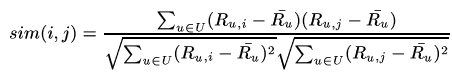
Pearson Correlation Coefficient

To solve above problem, we need to normalize the data by removing the bias before apply collaborative rating. (for each row, remove the average of the non-zero ratings of current row) and then adapt cosine similarity.

In short, it means that we check whether two users both agree that certain movie is above average. Based on this idea we could build a similarity matrix and then make recommendation.

The Delta

PROBLEM: 假设一个positive rating user与一群negative rating user有着相同的taste，那么根据CF我们可以向该user根据那群negative user推荐item I，但是I的rating由于是从negative user中得到的，故评分会比较低，那么这个评分对于该positive user可能会比较低。

Our goal, now, is to estimate the delta between my average rating and the others average ratings. Delta is (the difference between the rating that I estimate for item i on user u and the average rating of user u). Delta of u is equal to the summation of the delta of user v, times the similarity between v and u, divided by the summation of the similarities.

Item-Based Collaborative Filtering

IBCF

The item-based collaborative filtering is a symmetric approach to user-based. The only input is URM. We consider two items are similar if a lot of usrers share the same opinions on them.

In case we only consider implicit ratings, we take two columns from the matrix and measure the cosine of the angle between them.

IBCF explicit ratings

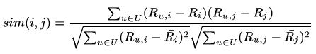
If we still use the cosine of the two vectors, it means we make a computation over u on the rating that user u gave to item i, times the rating that user u gave to item j, divided by the square root of the rating that user u gave to item i squared, times the rating that user u gives to item j squared.

The adjusted cosine

Problem 1 of cosine similarity: as an example, take any pair of movies: most of the users will have not rated these movies, so most of the ratings are zero. Now, suppose that there are two movies and I am the only person who rated them, rating both with five: I liked both of them. The cosine between these two movies will be of one, because all users who rated these two movies, which is only me on the rating. So, we are claiming the two movies are identical based only on the opinion of one user. Of course we cannot trust this.

We add a shrink term to the denominator of cosine formula to solve this problem.

Poblem 2 of cosine similarity: prositive users vs negative users

We apply the adjusted cosine: summation over the users of the rating that user u gave to item i, minus the average rating of the user, times the summation over u of the rating that user u gave to item j, minus the average rating of the user, divided by the square root of the summation of the ratings that user u gave to item i, minus the average of user ratings squared, times the summation over u, of the ratings that user u gave to item j, minus the average of the ratings of user u squared, plus the shrink.

Some considerations about CF

Normalization

Normalization is important if your goal is to estimate the rating, but, if the quality metric is an error metric or an accuracy metric, experience is telling us that you can safely remove the normalization without affecting the quality.

K-nearest neighbours

Save memory and time.

Choosing between user-based or item-based CF

IBCF is better than UBCF. For the following reasons

1. It is very difficult to find users similar to a given user. The computation of similarities between users is normally a problem because most of them will be zero. While, on the contrary, if you take two items and you try to see if there are users who rated both items, this probability is a little bit higher.
2. UBCF are not robust. If I rate a few new movies, it is very likely that the similarity between me and the other users will change dramatically.
3. If you have enough ratings that prove the two items are similar or dissimilar, even if you add more ratings, this similarity will not change much. In an item-based approach you can keep a model like this, without updating it for a lot of time. If you want, you can update the similar matrix once a day or a week or a month. From the practical point of view, it is impossible to create a real commercial recommender system that use a user-based approach on a large catalog of users and items. The performances are too low because you need to update continuously the model. It is time consuming.

Association Rules

The idea is to explore the data that you have in order trying to estimate the probability that something happens if something else happened in the past.

KEY IDEA: if you like i, there is great possibility that you will like j.

CONFIDENCE/SUPPORT/ASSOCIATION RULES/…